ITS ePrimer
Module 9: Supporting ITS Technologies
Authored by Brody Hanson, Research Associate, University of New Brunswick, Fredericton, NB, Canada
2014
Table of Contents
Purpose
Data collection, weather and traffic monitoring, communication, information dissemination, and in-vehicle systems are all essential components of intelligent transportation systems (ITS). The technology behind these components is a primary driver of effective ITS. Advances in technology and integration provide significant opportunities for system enhancement, so it is important to have an understanding of these technologies when considering an ITS deployment. This module provides an overview of various support technologies and considers opportunities for deployment and integration.
Return to top ↑
Objectives
Intelligent transportation systems are often described in terms of their application from a functional perspective; that is, what the overall system does. From the perspective of providing an overview of supporting technologies, this approach can make isolating specific technologies or ensuring a comprehensive overview difficult. Technologies that support ITS can have multiple functions within the same system or across different systems. Technologies that provide similar functions may not be suitable for similar applications.
The information in this module is organized so that each section has a specific focus facilitating the presentation and comparison of technologies. The takeaways from this section should be an understanding of:
- The various physical components of ITS.
- The different types of hardware technology used in each component.
- The strengths/limitations of comparable technologies.
- The example applications of supporting technologies.
Return to top ↑
Introduction
While other modules in this ePrimer focus on the application side of ITS, this module presents the actual equipment and technologies used to enable these applications. The module is broken down into sections that try to encapsulate and group the various physical components of ITS so that the different types of technologies can be compared and understood. The breakdown of supporting ITS technologies, along with a brief outline of each section, is as follows:
| Vehicle Detection |
This section discusses the various vehicle detection technologies used in ITS applications. This includes point detection technologies, such as inductive loops, radar, laser, video image processing, light-emitting diode (LED), infrared), and magnetometers. This also includes vehicle probe technologies, such as Bluetooth/Wi-Fi readers and cellular telephones. |
| Vehicle Monitoring and Tracking |
This section discusses the various vehicle monitoring and tracking technologies used in ITS applications. This includes technologies, such as, global positioning system (GPS), transponders/radio frequency identification (RFID), and license plate readers. |
| Communications |
This section discusses the various communications technologies used in ITS applications. This includes current wired technologies, such as fiber-optic and Ethernet cables, and leased telephone lines and cables. This also includes wireless technologies, such as spread-spectrum radio, Wi-Fi/ Worldwide Interoperability of Microwave Access (WiMAX), and cellular data. |
| Central Hardware and Systems |
This section discusses the various back-end technologies that are required in ITS applications. This includes distributed field controllers, central system hardware, and operating systems. |
| Dynamic Message Signs |
This section discusses variable message signs used to disseminate information in ITS applications. This includes fixed and portable dynamic message signs (DMSs). |
| Video Cameras |
This section discusses the video camera technology used to monitor traffic and transit. This includes standard cameras, dome cameras, Internet Protocol (IP) cameras, and on-vehicle cameras. |
| RWIS |
This section discusses the technologies used in Road Weather Information System (RWIS) applications. This includes a camera, road surface/subsurface sensor, and the various atmospheric sensors (e.g., temperature, wind, etc). |
| Connected Vehicle Technologies |
This section discusses the technologies used in connected vehicle (CV) concepts. This includes vehicle-infrastructure integration and communications technologies, such as dedicated short-range communications (DSRC), and vehicle-to-vehicle technologies (V2V), such as blind-spot detection systems. |
| Summary |
This section will provide a general summary and discuss some of the future technology issues and trends, such as new data sources, standards, and trickle-down technology. |
Each section offers typical or example implementations for the technologies discussed. Multimedia examples are also included, where appropriate, to assist with understanding and to provide context.
This module contains several private sector examples of supporting ITS technologies because the private sector is a common source of innovative supporting technology. The examples described are not an endorsement or advertisement for any one vendor.
Return to top ↑
Vehicle Detection
Vehicle detection is a cornerstone of most transportation applications. In the simplest form, the detection of vehicle presence has been widely implemented for decades, most notably at signalized intersections that regulate traffic lights based on traffic demands rather than pre-timed intervals. Advancements in technology have allowed for a dramatic increase in the type of vehicle characteristics that can be detected or determined, and have expanded the manner in which this data can be applied to improve the transportation network. In addition, a myriad of equipment types and topologies has enabled engineers to navigate infrastructure constraints and get traffic data in locations or situations at levels never thought possible. This section explores the technologies used in the detection of vehicles.
Point Detection
This section will investigate the various types of point detection technologies used and relied on in ITS applications. These detectors are intended to capture all of the traffic moving through the detection zone. This is different from probe detection (explored in a separate section) where only a subset of vehicles can currently be detected. Point detection refers to the detection of a vehicle at a single specific location (e.g., over an inductive loop). Some technologies can facilitate multiple detection points with a single detector by monitoring a zone or specified area (e.g., within the field of view of a video camera) and detecting when a vehicle has entered a certain point in the zone. These concepts will be explained in greater detail as the various technologies are presented. Although ultrasonic and acoustic detectors fall under this category, they are omitted due to their limited deployment in recent years.
Inductive Loops
The inductive loop method of vehicle detection is by far the most prevalent type of detection used in the United States. The technology has been in use since the 1960s, but is still worth reviewing given its importance as a component in many ITS applications. The following section provides an overview of how these detectors work.1
An inductive loop vehicle detector (or vehicle detector amplifier) system consists of three components: a loop (preformed or saw-cut), loop lead-in (or extension) cable, and a detector, as shown in the following diagram:
Figure 1. Inductive Loop Diagram
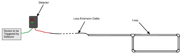
(Extended Text Description: This is a diagram of an inductive loop. Starting on the left, there is a gray box labeled "Device to be Triggered by Detector." A green line goes from this box, to a dark gray box labeled "Detector." There are two small indicators on the detector, one red and one green. From the detector, a red line comes out, and then joins with a black line. The black line goes from being solid to dashed, and back to solid. This is identified as a "Loop Extension Cable." The loop extension cable connects to a structure made up of five lines and four joints in the shape of a larger rectangle loop. This structure is initially straight, and is connected to a loop made up of the remaining four rectangles and joints.)
The preformed or saw-cut loop is buried in the traffic lane. The loop is a continuous run of wire that enters and exits from the same point. The two ends of the loop wire are connected to the loop lead-in cable, which in turn connects to the vehicle detector. The detector powers the loop causing a magnetic field in the loop area. The loop resonates at a constant frequency that the detector monitors. A base frequency is established when there is no vehicle over the loop.
When a large metal object, such as a vehicle, moves over the loop, the resonant frequency increases. This increase in frequency is sensed and, depending on the design of the detector, forces a normally open relay to close. The relay will remain closed until the vehicle leaves the loop and the frequency returns to the base level. The relay can trigger any number of devices, such as a gate, a traffic light, etc.
There is a misconception that inductive loop vehicle detection is based on metal mass. Detection is actually based on metal surface area. The greater the surface area of metal in the same plane as the loop, the greater the increase in frequency. Similarly, the frequency increases, as the metal surface gets closer to the loop, explaining why, in general, a compact car will cause a greater increase in frequency than a full-size car or truck. To this end, some success has been made with assigning a magnetic pattern to a particular vehicle and tracking that vehicle through a series of inductive loop detectors.
Loops are typically the most cost-effective detection option and are fairly reliable. They are, however, an intrusive type of technology meaning they are installed in the pavement or just below the pavement surface. This also means they are subject to external factors, which may cause damage. Pavement resurfacing, for example, requires the reinstallation of the in-ground component of the loop. Snowplows have also been known to cause damage to pavement, which in turn, may damage the loops. Loops are typically not installed in bridges or other areas where the road surface is sensitive.
The in-ground portion of the loop must be installed within a reasonable proximity of the detector (usually located in a roadside traffic controller cabinet). Distances approaching and exceeding 2,000 feet are subject to signal loss and degraded performance. Accuracy can also be compromised if the detectors are not calibrated properly or if lane changing in the detection area is common as vehicles may be counted in two lanes simultaneously.
When installed in a lane and separated by the appropriate distance (10 feet), these detectors can provide sufficient information to determine vehicle speed and length, which can be combined with other characteristics, such as volume and occupancy (i.e. the percentage of time a vehicle occupies the space over the loop; not the number of occupants in the vehicle) to form useful input into ITS applications.
Radar
Radar vehicle detection, shown in Figure 2, is a nonintrusive type of technology that uses microwaves to detect the presence of vehicles. Microwaves emanating from the device will reflect off of the metallic surface of the vehicle and, when properly calibrated, can provide the position of the vehicle relative to the device (e.g., which lane it is in). When two radar beams are used in series, characteristics, such as vehicle speed and length, can be obtained. Dual-beam radar antennas can be housed in the same unit; meaning only one device is needed to obtain these parameters.2
Figure 2. Radar Vehicle Detection Unit
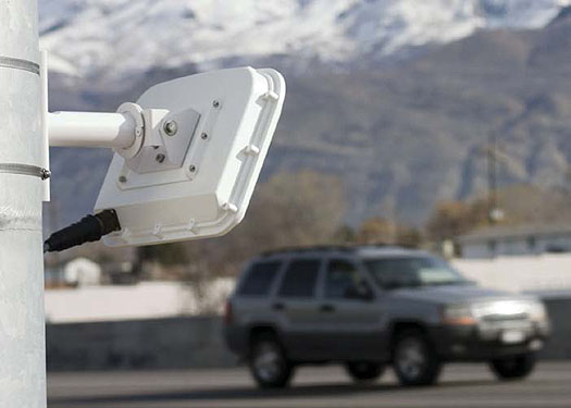
Source: Wavetronix.
Using the Doppler effect, radar devices can also detect vehicle speed based upon the change in frequency of the microwave reflected from the vehicle that is moving relative to the device. Typically, radar units are mounted in a side-fire configuration projecting across the traveled lanes, as illustrated in Figure 3.
Figure 3. Radar Detection Configuration
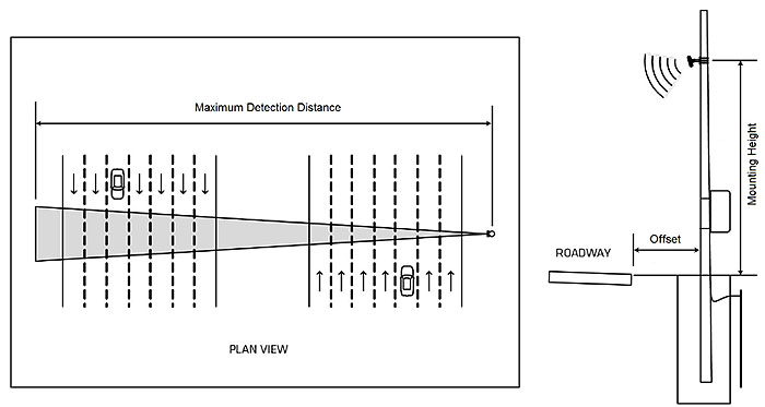
(Extended Text Description: This diagram is a Plan View showing the Maximum Detection Distance for a radar device. There are two sets of drawings of a seven-lane roadway oriented vertically. The seven-lane road on the left has a drawing of a car in the fifth lane, along with arrows in each lane pointing down. The seven-lane road on the right has a drawing of a car in the fifth lane, along with arrows in each row pointing up. On the far right of the diagram, there is a small square to represent a device. A triangular beam emanates from the device across all fourteen lanes of traffic. The distance from the small circle to the far end of the beam is labeled "Maximum Detection Distance.")
Source: Wavetronix.
Mounting height is usually a function of the offset distance from the roadway and specified by the manufacturer. A minimum of approximately 10 feet for the mounting height and 5 feet for the offset must be maintained to help ensure proper operation. These values also vary by manufacturer. Some success has been achieved using a zero offset configuration, but it is still recommended that the minimum offset be met.
Radar detectors are also available that operate in a front-fire mode, casting a footprint over a section of roadway, as illustrated in the following Figure 4.
Figure 4. Front-Fire Radar Detection Configuration
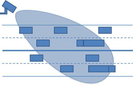
(Extended Text Description: This image represents the coverage area of a single radar device. In this image, there are rectangles representing vehicles in a drawing of a road with two lanes going in both directions. On the left there is a rectangular mounted device. From the device, a tear dropped oval is coming from the device and masks a portion of the roadway in blue. It does not cover all the cars depicted as driving on the road.)
Source: Brody Hanson Consulting.
Algorithms are used to continuously track vehicles that pass through the footprint. This way, information such as volume, speed, position (lane), and acceleration/deceleration can be determined.
Radar detectors perform fairly well during normal traffic conditions when installed within the guidelines provided by the manufacturer with regard to mounting height and offset. Performance tends to diminish during queued conditions, particularly with regard to lane occupancy. Occlusion is an issue with these devices and will cause some vehicles in the lanes farthest away from the detector to be missed, particularly if the units are not installed to meet the optimal height and offset requirements.
Radar detection devices are also prone to interference caused by nonvehicle metallic objects within the device's field of view. Reflections off of existing infrastructure, such as metal light standards, can cause the unit to behave erratically, thus compromising the data. Locations must be evaluated on a site-specific basis to ensure maximum accuracy. When properly located, installed, and calibrated, volume accuracies of up to 95 percent are achievable from this class of device. Environmental conditions such as wind, snow, or rain can have an effect on detection accuracy.
Laser
Vehicle detection using laser technology is available. The devices, shown in Figure 5, provide volume, lane occupancy, speed, and vehicle length data used in ITS applications.2
Figure 5. Laser Vehicle Detection Units
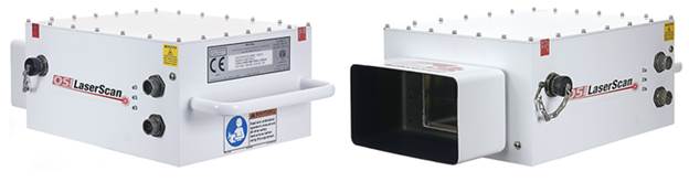
Source: OSI Laserscan.
The devices are designed to be installed directly above the travelled lanes, as shown in Figure 6.
Figure 6. Laser Detection Configuration
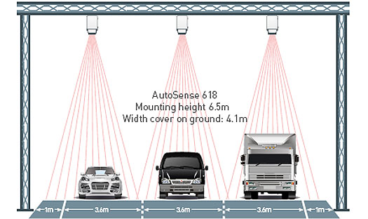
(Extended Text Description: This diagram shows icons of a sedan, a minivan, and a cargo truck side-by-side on three lanes of road underneath laser devices mounted overhead. There are three mounted devices, one to cover each lane. Laser beams depicted as a series of radiating lines shine down on each vehicle in a conical formation to cover to full width of each lane. Each lane of road is 3.6 meters with 1 meter of shoulder on both sides of the road. In the center of the model is the following text: "Autosense 618, Mounting Height 6.5 meters, Width cover on ground: 4.1 meters.")
Source: OSI Laserscan.
Figure 7. Video Vehicle Detection Unit
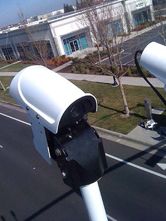
Source: Econolite Group, Inc.
Overhead laser detection technology is known to be quite accurate in all traffic conditions. The accuracy of the laser devices allows for the detection of vehicle profiles. For this reason, laser detection devices are popular in the tolling industry, where added parameters, such as vehicle height and tow-bar detection can be used to reinforce the vehicle classification.
Performance of laser-based detection systems begins to deteriorate during adverse weather conditions, such as snow, fog, and heavy rain. The magnitude of deterioration depends largely on the intensity of the adverse conditions, making this a potential concern for regions that experience high variability in weather conditions.
In general, the overall cost of implementing laser detection systems is higher than other systems. This is in part due to the fact that one device is required per monitored lane, and because an overhead gantry is required for their installation. Ideal locations for laser detection devices include locations where overhead infrastructure already exists, where other detection devices aren't suitable (e.g., a steel structure bridge where inductive loops cannot be installed in the bridge deck and the large amount of steel would cause reflective interference with radar devices), or where a high degree of accuracy is required.
Video Image Processing
Vehicle detection can be accomplished using video images taken from a video camera. The video images are sent through a digital signal processor to determine the presence of vehicles within the camera's field of view. An example installation is shown in Figure 7.
This device can be configured to provide the necessary type of data collection required for ITS applications, including volume, lane occupancy, speed, and vehicle length on a lane-by-lane basis.2
A camera is used to capture vehicular movement and presence within the travelled lanes. The recommended location to install cameras for this purpose is over the center of the travelled lanes, pointing against the flow of traffic, as shown in Figure 8.
Figure 8. Video Detection Field of View
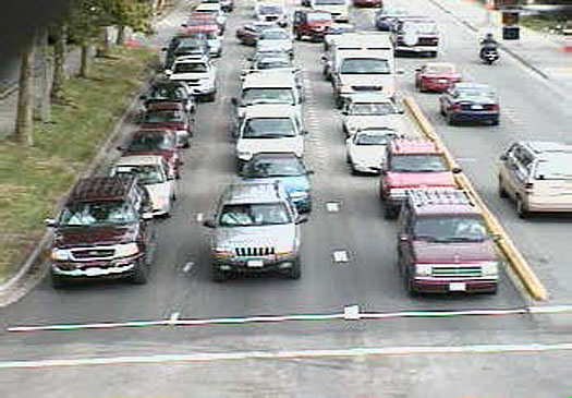
Source: Econolite Group, Inc.
Cameras should be installed as high as possible to reduce occlusion. Manufacturers usually provide minimum mounting height requirements. Once the camera has been installed, detection zones can be configured to provide point detection at the desired locations, as demonstrated in Figure 9.
Figure 9. Video Detection Zones
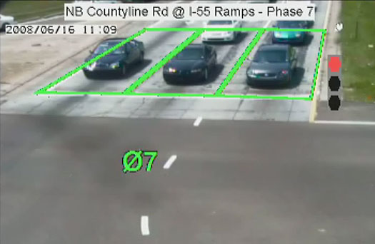
(Extended Text Description: This is an example of images from a video camera sent through a Video Image Processing Unit. In this image, there are three lanes of traffic waiting at an intersection. Lane space occupied by the first vehicles in line are outlined in green. To the right is an icon of a stoplight with the red light highlighted. At the top of the image is the location of the photo as well as the light phase.)
Source: Econolite Group, Inc.
The typical applications of video-based vehicle detection include presence detection at signalized intersections and incident detection along freeways. In these applications, video detectors have proven to be quite reliable. The devices can also be configured to emulate traditional inductive loops, facilitating their incorporation into other ITS algorithms and applications. An increasing number of jurisdictions have turned to video image processing to perform intersection movement counts. Portable cameras can be deployed to capture a video of the intersection over the counting period. The video is then uploaded to a central server location where it is processed and the turning movement counts are produced automatically.
One of the requirements for proper operation of the video-based detection system is a stable video feed. Vibration or camera sway can cause issues in the digital image-processing component of the system, which will significantly degrade performance. Visibility is also a cornerstone to the proper function of video-based detection systems. When the visibility is compromised, during heavy snow or fog for example, the performance of the system may be compromised. Adverse effects caused by differing light conditions and headlights may reduce the accuracy of the detectors. Natural impediments, such as overgrown trees or animals (e.g., birds), can also directly affect detector function (particularly in rural deployments).
An emerging technology in video image processing for vehicle detection is the use of thermal cameras. These cameras operate by detecting the heat signatures given off by everything in their field of view. This provides the potential for mitigating traditional video imaging issues, such as headlight blooming, glare, snow, and fog. This technology is still being proven in ITS applications.
Magnetometers
Microloops and wireless magnetometers are based on the same technology. They are similar to traditional inductive loops in that they provide point detection but differ by measuring changes in the earth's magnetic field to detect vehicle presence. Since the devices are basically an alternative to a traditional inductive loop, the same resulting data (volume, lane occupancy, speed, and vehicle length) on a lane-by-lane basis can be determined.2
Microloops require a direct connection to a traditional traffic controller. The microloop sensor and cable are shown in Figure 10.
Figure 10. Microloop Vehicle Detection Unit
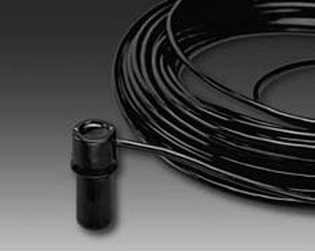
Source: Global Traffic Technologies.
Microloops are designed to be installed directly underneath the travelled lane as a replacement to a 6-feet by 6-feet inductive loop. In a typical roadway installation, a conduit is placed underneath the cross section of the roadway via directional boring at a standard depth from the road surface. The microloops are fed into the conduit and positioned such that they are in the center of each lane. The configuration for a bridge installation is fundamentally the same, except with a few additional constraints. The microloop is placed underneath the road surface in the center of the lane, at a specific depth, and at a minimum distance away from structural bridge members.
Figure 11. Wireless Magnetometer Vehicle Detection Unit
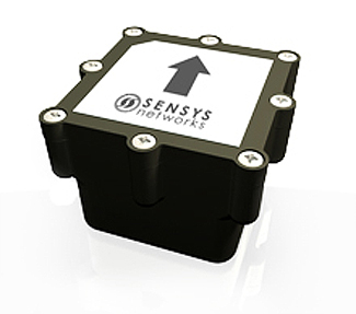
Source: Sensys Networks.
Most deployments to date have been installed in the typical under-roadway configuration. Initial results from the data analysis indicate that the devices produce similar results to inductive loop detectors but with some exceptions. Standard inductive loops typically can be installed at a distance up to 2,000 feet from a traffic controller. Microloops can begin to experience degraded performance between 1,000 to 2,000 feet. Also, lane occupancy levels tend to be much higher than that of a traditional loop (a nuance of differing technologies), but this can easily be adjusted for.
Wireless magnetometers (often called, puck-style detectors) are installed and configured to communicate wirelessly with an adjacent traffic controller and draw power from a built-in battery. Once installed, the detectors operate for a maximum period of 10 years before the battery runs down and the detector needs to be replaced. A wireless magnetometer is shown in Figure 11.
A single inductive loop is typically emulated by the installation of an array of puck-style detectors. The following video link provides additional information on wireless magnetometers and illustrates the actual installation procedure.
www.youtube.com/watch?v=4Eq-rcGd7kk (This video is set to private now.)
Infrared Detectors
Infrared detectors use infrared light cones sent from a transmitter to a receiver situated on opposite sides of the road perpendicular to the flow of traffic. These detectors can provide information, such as volume, speed, and classification data on a bidirectional, multilane roadway.3
This system consists of a receiver unit and transmitter unit placed on opposite sides of the road perpendicular to the direction of travel. Figure 12 shows a unit installed in the median.
Figure 12. Infrared Vehicle Detection Unit
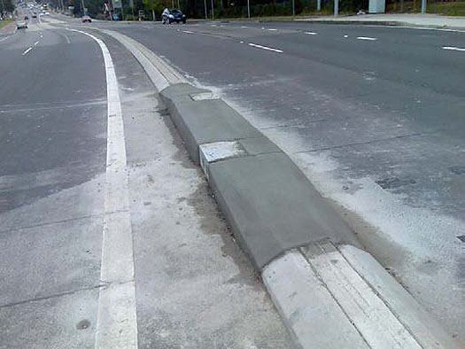
Source: CEOS Pty Ltd.
The transmitter sends two cones of infrared light across the roadway, and the receiver records vehicles as they break and remake these cones. The transmitter's infrared cones cross each other and form two straight and two diagonal beam pathways. When a vehicle crosses the beam pathways, the device records two beam events; it records one from the vehicle breaking and one leaving the beam pathway. These two beam events are recorded for all four beam pathways resulting in eight time-stamped events being generated per axle. The vehicle's velocity is derived from the time stamps of these beam events.
The interwheel (or interaxle) spacing can be determined since the velocity of each vehicle wheel is known and a time stamp is recorded for each axle crossing each beam. Once the interaxle spacing is known, it is compared to a table of interaxle spacing ranges stored in the unit to determine the correct classification of the vehicle. The results are stored on a per vehicle basis.
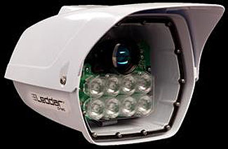
Figure 13. LED Vehicle Detection Unit
Source: Leddartech.
LED Detection
Vehicle detection can be accomplished using LED technology. These devices work by emitting light (either visible or infrared) via the diode and sensing the reflection in an optical sensor built into the unit based on the principle of the time-of-flight of light. Units are available that can be installed in a side-side fire configuration or in an overhead configuration. Figure 13 provides a close-up view of a unit's internal components, including the array of light-emitting sources and the optical sensor.
These detectors can provide volume and vehicle profile information and are often used for intersection stop-bar detection (where presence is important) or in tolling applications (where vehicle profile/classification is important). This technology operates independently of ambient lighting conditions and is not adversely affected by snow, rain, or fog. According to an LED detector manufacturer these devices can achieve a detection rate of greater than 98 percent.4
Probe Detection
This section will investigate the various types of probe detection technologies used in ITS applications. Wireless signals from vehicle embedded infotainment devices and/or driver/passenger wireless devices make it possible to detect the same vehicle at different locations in the road network, enabling applications such as travel time recording and origin/destination tracking.
Under current technology, these detectors capture a portion or subset of the traffic moving through the detection zone. This is different from point detection (explored in the previous section) where all the vehicles passing through the detection zone can be detected. Vehicle probe detectors can only detect vehicles if they contain a specific technological identifier. Consider the analogy of shopping at the grocery store. At the computerized checkout, the computer can automatically determine the presence of a product in a shopping cart by using the barcode scanner to read the product's barcode. This only works if the product has a barcode identifier. For the many products that don't have this identifier (e.g., produce), passing the product through the barcode scanner will have no effect as the computer has no way to automatically detect the product. This is, in essence, the same as the vehicle probe concept. Vehicles passing through the detection zone will not be detected if they don't possess the technological identifier.
Cellular Telephones
The activity of using cellular telephones as a means to determine traffic characteristics has become increasingly effective with the increased use of the devices. Systems that use cell phones to wirelessly locate travelers can be classified into two general groups: handset-based systems and network-based systems.5 Handset-based systems rely on GPS-enabled wireless phones. The GPS unit in the handset determines the location of a phone, and this information is relayed from the phone to a central processing system maintained by the wireless carrier.
Network-based systems utilize signal information from cell phones to derive the location of the phone using cellular triangulation. Each phone can be identified by its electronic serial number, a unique number assigned to every phone that has been produced since cellular telephone technology was developed. In some cases, network-based systems require the installation of special equipment throughout a metropolitan area in order to analyze signal characteristics of calls. For example, some network-based systems determine positions by analyzing signal power and angle of arrival at multiple cellular towers. In other cases, network-based systems derive location estimates purely from signal information already available at cellular towers. Since network-based systems do not require users to have GPS-enabled phones, they generally provide less spatial accuracy than handset-based systems. This technology is also unique to each service provider, limiting the source of data to those phones serviced by the individual service provider.
The process of deriving traffic information from these data follows three basic steps. First, the location of the probe must be determined. These position estimates are usually inaccurate to some degree and may not lie directly on the roadway network. Second, the position estimates are matched to a specific road. Techniques for map matching vary from simple geometric methods to more complex statistical approaches that account for link connectivity and past travel history. Third, this data is aggregated and its characteristics are used to determine traffic speed and travel times for a given road link. The algorithms used in this process are highly complex and result in a portrayal of traffic conditions, which is generally fairly accurate. Accuracy increases/decreases as the number of cell towers in the area increases/decreases.
One of the biggest limiting factors with using cellular telephone probes is the number of samples available at any given time. Just because there is a cell phone inside a vehicle does not mean the vehicle represents a valid sample. In order to derive the necessary information, the cell phone must be active. That means, for GPS-based phones, communication of the device's location and speed/direction must be given to the network provider, which occurs when the cell phone user initiates a GPS location query (e.g., viewing the user's location on a map using a smartphone or opening an app that provides map-based traffic information). For network-based systems in current deployments, phones must be transmitting/receiving (e.g., the user is engaged in a telephone call).
Bluetooth and Wi-Fi Sensor Networks
Bluetooth is a telecommunications industry specification that defines the manner in which mobile phones, computers, personal digital assistants, car radios, and other digital devices can be interconnected using short-range wireless communications. Bluetooth uses a low-cost transceiver chip to exchange information with other Bluetooth devices within a globally available frequency band of 2.45 GHz.6 A few years ago automobile manufacturers began increasing embedded Bluetooth technology into their infotainment systems so that drivers could connect their phones or music devices to the vehicle for control and play. Smartphones, which today form more than 60 percent of the installed base of cellular phones in North America, also include Wi-Fi wireless technology for higher speed connection to Wi-Fi base stations for email, video, etc.
Both Bluetooth and Wi-Fi transceivers regularly broadcast "discovery" messages as the devices look for networks or other devices with which to connect. The devices broadcast unique identifiers in these messages, which are not traceable to an individual and, with proper management, meet privacy legislation requirements. This creates a unique opportunity for data collection, in that a Bluetooth or Wi-Fi sensor placed close to a roadway can detect devices inside passing motorists' vehicles. Roadside sensors read these Bluetooth and Wi-Fi messages and record the time at which the device passed by the sensor. Each sensor either stores locally (for postprocessing) or reports (provided communications are available) the identifier and the time to a central server. The data for each device across two or more sensors can be matched up to calculate travel times and traffic speeds for each segment between sensors, travel times across multiple segments within the network, and origin/destination pairs. This is illustrated in Figure 14.
Figure 14. Bluetooth Travel Time System Illustration
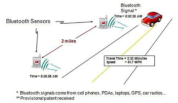
(Extended Text Description: This is a diagram illustrating Bluetooth sensor coverage on a road. In the diagram there is a vehicle driving down a road. On the left side, there are two Bluetooth sensors placed alongside the road. Distance been the sensors is two miles. As the vehicle approaches the first sensor, a Bluetooth signal timestamp 8:03:26AM is recorded. A timestamp of 8:05:58AM is recorded at the second Bluetooth Sensor. The travel time and speed calculated are 2:32 minutes and 51.7 MPH. At the bottom of the diagram, are the following notes: "Bluetooth signals come from cell phones, PDAs, Laptops, GPS, Car radios… " and "Provisional patent received.")
Source: Traffax Inc.
Advanced algorithms eliminate outliers, such as pedestrians or cyclists carrying devices, delivery vehicles making stops, or buses carrying many people with many devices. These sensors can also be used to anonymously track transit users or pedestrians along their route or across multiple modes, providing origin destination and mode shift information to agencies.
As with any probe detection technology, the penetration rate of vehicles containing these devices is often a governing factor in the timeliness and accuracy of the resulting data. Penetration rates for Bluetooth in nonurban, noncommuter areas are typically around 5 percent, while in urban commuter corridors these rates are typically 20 to 25 percent during peak periods. The proliferation of hands-free legislation has increased the uptake of Bluetooth-enabled cell phones but, at the same time, newer smartphones (e.g., Android and iPhone) have changed the default Bluetooth setting to off, meaning discovery messages are only broadcast when devices are pairing. Built-in Bluetooth devices in automobiles still broadcast regularly.
Smartphones constantly search for new Wi-Fi networks, but the discovery broadcasts are much less frequent than Bluetooth. This reduces penetration, particularly for vehicles travelling at high speeds. A newer strategy combines the Bluetooth and Wi-Fi sensors into one device to maximize the overall penetration rate. According to a manufacturer, this new strategy makes it possible to detect up to 50 percent of vehicles.
Systems using these technologies in a real-time context have to account for the inherent latency that is built in to this data collection method. For example, the most current recorded travel time for a particular road link is based on the last detected vehicle to exit the system. This information may no longer be relevant to vehicles entering the road link since conditions may have changed in the time it took the last detected vehicle to travel through the system. This can be mitigated by physically spacing detectors closer together or with software that adds a predictive element using additional data gathered from other parts of the system.
Return to top ↑
Vehicle Monitoring and Tracking
Before discussing vehicle monitoring and tracking technologies, the difference between this and vehicle detection should be clarified. Vehicle detection, as presented above, focuses on detecting the presence and/or characteristics (e.g., speed) of vehicles in general. That is, there is no interest in the specific vehicle itself, only the vehicle's presence/characteristics. Vehicle monitoring and tracking, on the other hand, focuses on detecting (and tracking) a specific vehicle. In these applications, agencies are interested in the characteristics (e.g., location) of specific vehicles (e.g., buses) for a variety of reasons. This concept will be explained further as the various technologies are presented.
GPS
GPS tracking is a method of electronically determining an object's location in terms of latitude and longitude based on signals received from multiple GPS satellites. GPS is mainly funded and controlled by the United States Department of Defense (DOD). The system was initially designed for the U.S. military; today, there are also many civil users of GPS throughout the world. Civil users are allowed to use the standard positioning service without any kind of charge or restrictions.7
GPS tracking is a method of working out exactly where something is. A GPS tracking system, for example, may be placed in a vehicle, on a cell phone, or on special GPS devices, which can either be fixed or portable units. GPS works by providing information on exact location. It can also track the movement of a vehicle or person. So, for example, a company can use a GPS tracking system to monitor the route and progress of a delivery truck or the location of high-valued assets in transit, and parents can use a GPS device to check on the location of their child.
A GPS tracking system can work in various ways. From a commercial perspective, GPS devices are generally used to record the position of vehicles as they make their journeys. Some systems store the data within the GPS tracking system itself (known as passive tracking), and some send the information to a centralized database or system via a modem within the GPS system unit on a regular basis (known as active tracking) or 2-Way GPS.
A passive GPS tracking system will monitor location and will store its data on journeys based on certain types of events. So, for example, this kind of GPS system may log data such as where the device has traveled in the past 12 hours. The data stored on this kind of GPS tracking system is usually stored in internal memory or on a memory card, which can then be downloaded to a computer at a later date for analysis. In some cases, the data can be sent automatically for wireless download at predetermined points or times, or can be requested at specific points during the journey.
An active GPS tracking system is also known as a real-time system as this method automatically sends the information on the GPS system to a central tracking portal or system in real time as it happens. This kind of system is usually a better option for commercial purposes because it can be used to track a fleet or monitor people. Caregivers who use the system to monitor children or elderly can know exactly where loved ones are, whether they are on time, and whether they are where they are supposed to be during a journey. Transit agencies can use real-time GPS systems to track transit vehicles along their routes. Advanced systems use this information for traveler information purposes by relaying the position or anticipated arrival time for wayside or website dissemination.
Transponder and RFID-Based Tracking
A basic RFID system consists of tags, antennas, and readers.8 The reader's radio frequency (RF) source is either integrated or a separate component. The reader broadcasts RF energy over an adjustable area called the read zone or reader footprint. The tag on the vehicle reflects a small part of this RF energy back to the antenna. The reflected radio waves denote the tag's unique identification code and other stored data. The antenna relays the signal to the reader, which can add information, such as date/time to the tag's identification code, and stores it in a buffer. The reader can transmit the tag's identification code to the customer's information management system. Most ITS applications use active in-vehicle transponders rather than passive RFID tags (common in freight tracking applications). These transponders use a battery-powered transceiver to emit the unique identifier when the device passes through the reader footprint. The entire process takes only milliseconds.
RFID transponders and their associated readers are a core component of electronic toll collection (ETC) systems used by toll agencies across the nation. Transponders associated with user accounts allow customers to pay tolls without using cash, which improves traffic flow at toll plazas. Some agencies have adopted open road tolling, which allows tolls to be collected at highway speeds.
RFID transponders can also provide a probe data source for calculating travel times in regions with a high penetration of toll transponders in vehicles. In these applications, the transponder IDs are encrypted by the travel time system to mitigate privacy concerns and regulations. The result is an approach that is fundamentally the same as that used by Bluetooth/Wi-Fi sensor travel time systems (discussed in a previous section) where a unique identifier is time-stamped at multiple locations facilitating the derivation of travel times and link speeds. This also means that this approach is subject to many of the same constraints, e.g., penetration rates and inherent latency, as the Bluetooth/Wi-Fi sensor systems.
License Plate Readers
License plate readers, also known as automated number plate recognition (ANPR) systems use cameras to read the license plate number on vehicles at each detection point in a road network. License plate recognition involves capturing photographic video or images of license plates, whereby they are processed by a series of algorithms that provide an alphanumeric conversion of the captured license plate images into a text entry.
The following link contains an animation that demonstrates this process:
www.licenseplatesrecognition.com/how-lpr-works.html- content is no longer available.
The presence and time of a specific vehicle along with a time stamp are sent to a central server and processed. This technology lends itself especially well to toll collection with high volumes of traffic in a single direction and where evidentiary proof may be necessary. In these applications, readers are located at the entry/exit points to the toll highway. Vehicles are identified as they enter the highway and as they leave facilitating the calculation of tolls based on the distance travelled on the toll road. ANPR is often used in tolling to supplement a primary vehicle identification method, such as RFID transponders. The technology can also be used to provide travel times and link speeds in the same manner as RFID/Bluetooth/Wi-Fi technologies (discussed in previous sections).
Return to top ↑
Communications
Advancements in the global communication networks and technologies have been one of the greatest enablers of ITS applications. Internet-connected devices and Web-enabled applications provide a robust environment in which to develop transportation-related applications. That said, ITS still needs to interface with the outside world and its associated constraints, meaning the design of the communication system for ITS is far from trivial. The various communication technologies used in ITS applications are discussed here.
Wired Communications
Fiber-Optic Cable
The basic principle behind fiber-optic technology is that light pulses are transmitted along an optical cable, similar to how electrical signals are sent along copper cable. An optical transmitter and optical receiver at each end of the optical fiber convert electrical signals into light signals that are transmitted along the optical fiber. In its most rudimentary form, a point-to-point fiber- optic transmission system can be created by connecting a transmitter and receiver together with some fiber-optic cable.9
Fiber-optic cable provides the highest bandwidth of any current communications system. This is extremely useful for ITS applications where large amounts of data are transmitted, such as video. A typical industry bandwidth rate for fiber-optic cable is 1.5 gigabits per second (Gbps). The technology also offers low attenuation, meaning cable runs can be quite long (several miles) before amplification is required.
All fiber-optic cables have a glass core. The core is surrounded with optical cladding (also glass), which stops the light escaping by using the principle of total internal reflection (or refraction). The remainder of the cable is a layered mixture of various materials to provide protection from the environment and from physical damage.
Figure 15. Fiber-Optic Cable Diagram
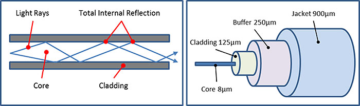
(Extended Text Description: There are two diagrams in this image. On the left is an illustration of how light travels down a fiber optic cable. The fiber optic cable is shown as a white tube in between gray rectangles representing cladding on top and on the bottom. Within the fiber optic line, blue lines represent light rays bouncing off the walls of the cable. The point at which the light ray hits the clad is called "Total Internal Reflection." The very center of the fiber optic cable is called the core. The diagram on the right shows how a fiber optic line is packaged. In the very center is 8um of fiber optic core. The core is surrounded by a 125um cladding. Around the cladding is 250um of buffer. And finally surrounding the buffer is a 900um thick jacket.)
Source: Brody Hanson Consulting.
Since data is transmitted using light, electrical resistance and contact corrosion are not a concern. Light is not susceptible to magnetic interference so the cables require no electrical screening. All fiber connectors have dust covers because even small amounts of dirt and dust will interfere with the light transmission and cause losses.
Fiber-optic cable comes in two forms: multimode and single-mode. Multimode fiber has a relatively large light-carrying core, usually 62.5 microns or larger in diameter. It is usually used for short-distance transmissions with LED-based fiber-optic equipment. Single-mode fiber has a small light-carrying core of 8 to 10 microns in diameter. It is normally used for long-distance transmissions with laser diode-based fiber-optic transmission equipment.
In ITS applications, multifiber cables are common. The optical-fiber buffers are typically bundled inside buffer tubes, which are then bundled inside the larger cable. Optical fibers and buffer tubes are color-coded to allow for consistent splicing to adjacent cables. It is common to find 12-count, 24-count, and 72-count fiber-optic cables (among others) in ITS applications. Cable construction will vary depending on whether the cable is intended for aerial installation, installation in a buried conduit, or in a direct-bury application.
Traditionally, fiber-optic cable is considered an expensive option. The proliferation of its use in many different industry sectors has driven down the cost of fiber-optic cable to a point where the relative cost versus other wired media is comparable; particularly for new installations where trenching is the largest component of the cost. Fiber-optic cable can be expensive to repair if damaged, as highly specialized tools and expertise are required to mend a broken cable.
Twisted Wire Pair (TWP)
Twisted wire pair is still one of the most common methods of wired communications in traffic management systems. TWP cabling is a type of wiring in which two conductors of a single circuit are twisted together for the purposes of canceling out electromagnetic interference from external sources. The cables are typically shielded. This shielding can be applied to individual pairs or to a collection of pairs. When shielding is applied to a collection of pairs, this is referred to as screening. Shielding provides an electric conductive barrier to attenuate electromagnetic waves external to the shield and provides a conduction path by which induced currents can be circulated and returned to the source, via ground reference connection.
Traditionally, TWP was limited to slow serial communications. Advancements in technology have led to the widespread use of Ethernet over TWP in ITS and transportation management applications. This has facilitated the leveraging of legacy TWP infrastructure into current ITS by allowing the cables to carry the increased bandwidth required in systems today.
Ethernet Cable
Ethernet cables connect network devices, such as modems, routers, and adapters. They transmit data using the Ethernet protocol. Ethernet cables normally support one or more industry standards. Although Category 6 (CAT6) cable is becoming increasingly common, currently the most common standard is Category 5 (CAT5).10
CAT5 is an Ethernet network cable standard defined by the Electronic Industries Association and Telecommunications Industry Association (EIA/TIA). CAT5 is the fifth generation of twisted pair Ethernet technology and the most popular of all twisted pair cables in use today.
CAT5 cable contains four pairs of copper wire. It supports Fast Ethernet speeds (up to 100 Mbps). As with all other types of twisted pair EIA/TIA cabling, CAT5 cable runs are limited to a maximum recommended run length of 328 feet.
Although CAT5 cable usually contains four pairs of copper wire, Fast Ethernet communications only utilize two pairs. A newer specification for CAT5 cable (CAT5e) supports networking at Gigabit Ethernet (up to 1,000 ps) over short distances by utilizing all four wire pairs, and it is backward-compatible with ordinary CAT5.
Twisted pair cable like CAT5 comes in two main varieties, solid and stranded. Solid CAT5 cable supports longer-length runs and works best in fixed-wiring configurations like office buildings. Stranded CAT5 cable, on the other hand, is more pliable and better suited for shorter-distance, movable cabling, such as on-the-fly patch cabling.
Nearly always, 8P8C modular connectors, often referred to as RJ45, are used for connecting CAT5 cable. Most CAT5 cables are unshielded, relying on the twisted pair design and differential signaling for noise rejection. Each of the four pairs in a CAT5 cable has differing precise number of twists per foot to minimize crosstalk between the pairs.
In ITS applications, Ethernet cables are useful for connecting high bandwidth devices, such as video cameras, to a network or to an Internet access point. They are low cost, but the relatively small run length largely limits their application to anything other than local device interconnect. The following video from one of the creators of Ethernet provides an overview of the history and development of Ethernet technology: www.youtube.com/watch?v=g5MezxMcRmk
Power over Ethernet (PoE) describes a standardized system to pass electrical power along with data on Ethernet cabling. This allows a single cable to provide both data connection and electrical power to such devices as vehicle detectors and video cameras. Unlike standards such as Universal Serial Bus, which also power devices over data cables, PoE allows long cable lengths. Extra pairs of wire, not used for data transmission, are used for power. Up to 25 watts is available for a device, depending on the version of the standard in use. CAT5 (or higher) cable is required for PoE applications.
Leased Communications Systems
A popular option in the deployment of ITS is the use of leased communications services. Telecommunications companies have existing widespread communications networks that can allow transportation agencies to implement widespread connectivity to field devices without the need for large upfront capital expenses. Lease systems come in a variety of forms and technologies ranging from legacy to modern.
Leased telephone lines are considered a legacy type of technology. Most jurisdictions are moving away from this technology as it offers the lowest bandwidth of any communication medium and generally carries a high recurring lease cost. Communication via leased lines is achieved through use of a modem. A modem is required on each end of the transmission to send and receive communication information. The sending modem modulates the data into sound, and the receiving modem demodulates the sound back into data.
Maximum bandwidths are very low (19.2 to 56 kb/s) limiting the potential application of leased lines in the ITS realm. The largest adaptation of this communication medium has been in urban traffic control systems due to the low bandwidth requirements and the existence of widespread telephone infrastructure. Even during real-time applications, such as intersection monitoring and adaptive traffic control, these applications only require a small amount of data to be transmitted. Leased telephone lines can also provide options for rural ITS applications where cellular service is not available and installing a new communication line is cost prohibitive.
Digital subscriber line (DSL) is a family of technologies that improves the speed of communications over the wires of a local telephone network by using higher frequency bands for data. The bit rate of DSL services typically ranges from 256 kbps to 40 Mbps in the direction to the customer (downstream), depending on DSL technology, line conditions, service-level implementation, and distance from the service provider. DSL has a theoretical maximum operating range of 38,000 wire feet from the nearest DSL multiplexer.
Cable Internet is a form of broadband Internet access that uses the cable television infrastructure in the same manner that DSL uses telephone infrastructure. ITS devices are connected to a cable modem and communications are made through coaxial cable. The maximum bandwidth for cable Internet connections is 100 to 400 Mbps meaning it is suitable for most high bandwidth ITS applications.
One benefit that leased communications providers can offer is a Virtual Private Network (VPN). This extends a private network across public networks, like the Internet, in a secure manner. It enables a host computer to send and receive data across shared or public networks as if they were an integral part of the private network with all the functionality, security, and management policies of the private network. High bandwidths are achieved by Internet Protocol Virtual Private Networks (IPVPN) using Multiprotocol Label Switching (MPLS).
Wireless Communications
Figure 16. Spread-Spectrum Radio Configurations
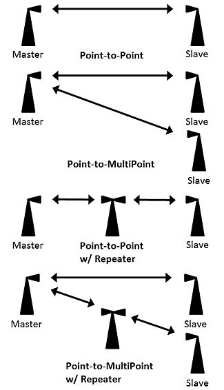
(Extended Text Description: This image depicts several spread-spectrum radio configurations. Point-to-point has an icon of tall triangle with a cone at the top, labeled Master, and another similar icon, labeled Slave, with a bi-directional arrow between the two icons. Point-to-Multipoint configuration has a Master icon with bi-directional arrows pointing to two different Slave icons. In the Point-to-Point w/ Repeater configuration has a Master icon with a bi-directional arrow pointing to an icon of a tall triangle with two cone shapes at its top, labeled the Repeater. This icon has another bi-directional arrow pointing to a Slave icon. In the Point-to-Multipoint w/ Repeater configuration has a Master icon with a bi-directional arrow pointing to a Slave icon, as well as to a Repeater icon that points to another Slave icon.)
Source: Brody Hanson Consulting.
Spread-Spectrum Radio
Spread-spectrum radios are becoming a popular communications option for ITS applications because they are fairly easy to implement. They do not require FCC (Federal Communications Commission) paperwork or licensing, which makes them easy to procure and install.11
Implementation of a radio network requires a transmission path study. Radio manufacturers can usually provide such studies. This study determines how many and where the radios will be installed and provides height requirements for antennas so that they can achieve the best line-of-sight communications.
The configuration of these radios follows standard network topology, not unique to spread-spectrum radios. A basic spread-spectrum communications link requires two radios, one radio acting as a master and the other as a slave. This is called a point-to-point system. If a master radio cannot communicate to a slave radio due to distance or interference, another radio (repeater) is installed between the two radios. The repeater, as the name implies, receives and resends the signal to the appropriate device(s). The repeater will be located at a point where it can communicate to all devices. Figure 16 shows the different methods of communicating over a radio (standard network topology applies). The following link provides an overview of how mesh Ethernet radios work (Click on Video 2).
www.encomwireless.com/encom-support/product-support/training-videos- content is no longer available.
Radios in ITS applications can broadcast over the unlicensed frequencies of 900MHz, 2.4GHz, or 5.8GHz. Radios broadcasting in the 900MHz frequencies provide the lowest throughput but are the least susceptible to line of sight issues. These radios offer serial throughputs of up to approximately 230 kbps and Ethernet throughputs of up to approximately 22 Mbps. Radios in the 5.8GHz range use Ethernet and provide the highest bandwidth of 54 Mbps and are most susceptible to line-of-sight issues. The use of lower bandwidths mitigates line-of-sight issues at the expense of data transfer rates, whereas the use of higher bandwidths maximizes data transfer rates but is more susceptible to line-of-sight issues.
An example of a typical spread-spectrum installation would be the connection of a series of traffic controllers at signalized intersections back to the traffic management center (TMC) for intersection monitoring and signal timing purposes. The TMC may install several high bandwidth 5.8GHz trunk lines to access traffic corridors throughout the city. Local intersections are typically interconnected using 900MHz serial radios due to their low bandwidth transmission requirements and ability to mitigate line-of-sight issues. Groups of these intersections would then be connected to an access point on the 5.8GHz network for transmission back to the TMC. This connection is made possible with the use of a terminal server, which is simply a device that provides the conversion of serial to Ethernet communications.
Line-of-sight issues tend to be the biggest limiting factor in the implementation of spread-spectrum radios. Theoretically, these types of radios can communicate at ranges of up to 60 miles. In practice, this distance is often limited to a few miles due to obstructions such as trees, buildings, or variations in topography. Similarly, the theoretical maximum bandwidth may be 54 Mbps, but the practical maximum is actually closer to 20 Mbps. This occurs because it is difficult to maintain a constant stream of communication at that level. That is, the radios will communicate in short bursts of up to 54 Mbps, but environmental interference prohibits a prolonged connection, resulting in a lower practical maximum. Also, since these frequencies are unlicensed, interference can be introduced from other public wireless devices operating at the same frequency.
Licensed trunk radio has been shown to provide an alternative to unlicensed spread-spectrum radio in certain ITS applications.12 This technology works like a packet switching computer network allowing multiple users to share the same channel but communicate with different radios. This option provides an extremely low bandwidth but has demonstrated success in providing communication to remote ITS components with a low bandwidth requirement (e.g., dynamic message signs).
Wi-Fi/WiMAX
Wi-Fi is a popular technology that allows an electronic device to exchange data wirelessly (using radio waves) over a computer network. Wi-Fi refers to any wireless local area network product that is based on the Institute of Electrical and Electronics Engineers (IEEE) standard 802.11. Wi-Fi typically provides local network access for around a few hundred feet with speeds of up to 54 Mbps. The main components of a Wi-Fi network are the wireless access point (WAP) and the wireless adapter. Wireless adapters allow wireless devices (e.g., smartphones) to connect to the WAP. The WAP connects wireless devices to an adjacent wired network. In order for the wireless devices to communicate with other wired devices, the WAP must be connected to a switch or Ethernet hub. If the WAP and switching hardware are housed in the same unit, the configuration is known as a wireless router.
Worldwide Interoperability for Microwave Access (WiMAX) is a wireless communications standard designed to provide high bandwidth at an extended range. It is similar to the Wi-Fi standard but on a much larger scale and at faster speeds. WiMAX refers to interoperable implementations of the IEEE 802.16 family of wireless networks. A WiMAX antenna can have a range of up to approximately 30 miles and offer speeds up to approximately 70 Mbps with newer versions of the standard aiming to provide 1 Gbps.
Cellular Data
In the 1990s, two primary cellular technologies, GSM (Global Systems Mobile) and CDMA (Code Division Multiple Access), were deployed by Mobile Network Service Operators (MNSOs) for the purpose of mobile voice phone calls. Over time, increasing data functionality was added from short message service (SMS) to data access to MNSO servers, to broadband mobile access to the Internet at large. The Internet function of cellular networks is based on Transmission Control Protocol (TCP)/Internet Protocol (IP), the language of the Internet, and synonymous with the Packet Data Protocol.13
A key difference between the two major cellular technologies is how they transfer the data for efficiency and speed. GSM technology divides the frequency bands into multiple channels so more than one user can send data through a tower at the same time; CDMA networks layer digitized calls over one another, and unpack them on the back end with sequence codes.
GSM and CDMA have both gone through series of evolutions, remaining primarily voice-call oriented but delivering increasing data and call density for the operators and higher potential data bandwidth for users. CDMAs evolved into evolution data only (EvDO), which has a theoretical download/upload speeds of 3.1/1.8 ps. GSM has grown into high-speed packet access (HSPA) with download/upload speeds of 7.2/5.76 Mbps. The newest GSM version, created to rival Long Term Evolution (LTE), is called Evolved HSPA (HSPA+) and boasts theoretical download/upload speeds of 42/11.5 Mbps.
LTE is the newest technology and is dramatically different from predecessor technologies. This 4G standard is designed to carry and manage broadband data streams with voice as an override. With data at its foundation, LTE offers spectral efficiency, high bandwidth (150/75 Mbps download/upload), the application and use of all the data management and security of IP networks, and low latency. LTE also supports full data rates while travelling at high speeds where GSM and CDMA experience degraded performance. LTE Advanced will be the next generation of technology using the LTE platform touting theoretical download/upload speeds of 1000/375 Mbps download/upload. All of these data rates are theoretical maximums; in practice, environmental factors contribute to actual speeds that are significantly lower, usually about half.
Deciding which technology to use is an exercise in determining the latency required, availability, coverage, and price. Latency, a measure of time delay in the system, can vary throughout the day due to varying network loads. Depending on the carrier and its strategy, each service provider has constantly evolving rate plans and packages for machine-to-machine data connectivity. Another dimension of service selection is security. This will determine whether general wireless Internet with the usual security mechanisms is sufficient or whether a managed VPN is required. Consideration should be given to the expected lifetime of the application in comparison to the carrier-specific expected lifetime for the cellular data technology. Many MNSOs are rapidly turning down older networks in order to utilize the spectrum for more modern technologies.
Return to top ↑
Central Hardware and Systems
Central Systems
Typical central systems consist of multiple servers (application, database, communications, video, etc.), workstations, communications media/interface, and displays (e.g., video walls).
Personal computers are still the most popular form of operator interface in TMCs today. Video walls (or video cubes) are becoming increasingly popular for traffic monitoring applications. One consideration that agencies often omit in contemplating a video wall implementation is the operational cost. Advances in display technology can mitigate this by incorporating long life lamps, LED light sources, and features including automatic color calibration. Maintaining uniform brightness levels and an appropriate contrast ratio are important factors in an effective video wall. Figure 17 shows video wall implementation in Bellevue, WA.
Figure 17. TMC Video Wall
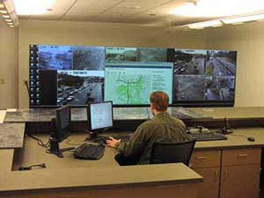
Source: City of Bellevue, WA.
The other main component of a TMC is the central server. Servers used in ITS applications are the same as those used across other industries in central server applications. The server acts as a platform on which the particular ITS application is built. It is the nerve center that provides the connection between the field equipment and the operator's interface. Server hardware is available from multiple manufacturers. Central software is available for a variety of operating systems, including Linux and Microsoft Windows servers. Large servers are located onsite in dedicated climate-controlled rooms along with other hardware, such as routers and switches, as well as other shared equipment for the organization.
Outsourcing of central system functionality is becoming increasingly popular. This is enabled through cloud computing and the provision of Software-as-a-Service (SaaS). Cloud computing is the use of computing resources (hardware and software) that are delivered as a service over a network (typically the Internet). This is an attractive option for some agencies as it can help avoid upfront hardware procurement and long-term maintenance costs. Since central hardware is stored and maintained offsite, there is less need for dedicated in-house IT staff or for dedicated space to store system hardware.
Field Traffic Controllers
Devices and sensors deployed in the field need some control mechanism or interface to integrate with an ITS. This is accomplished through the deployment of field controllers. The controller is the intelligence of the local system, providing a common point to connect, monitor, and control field equipment. Standard types of controllers are typically housed in a roadside cabinet.
Controllers and controller cabinets often operate with an uninterruptible power supply/source (UPS). This is an electrical apparatus that provides emergency power when the main input power source fails. This is extremely useful since many ITS applications are safety sensitive. A UPS differs from an auxiliary or emergency power system or standby generator in that it will provide near-instantaneous protection from input power interruptions by supplying energy stored in batteries. A UPS can allow equipment to operate for several hours without main power restoration, depending on the battery size and equipment configuration.
The majority of controllers in use today operate at signalized intersections, facilitating the safe and proper operation of traffic lights, pedestrian signals, and vehicle detectors. More robust controllers can facilitate advanced forms of traffic management, such as transit signal priority and adaptive traffic control. Other controllers provide a real-time operating system environment that can house advanced logic for applications, such as incident management or border wait time measurement. In some cases, the hardware and firmware for a controller can be procured separately. The four main types of commercial controllers are presented here.14
Type 170
California Department of Transportation (Caltrans) developed one of the first Type 170 specifications in the early 1970s, which specifies the form, fit, and function of the traffic controller hardware as well as many of the hardware design elements, including the required use of a specific 8-bit microprocessor. The specification also covers the cabinet-controller interface, including the shape and size of the controller itself. Particularly, the 170 specification covers the need to fit the controller into a 19-inch standard rack. A key element of the 170 controller is that it uses discrete inputs and outputs to interface with the traffic control cabinet. This is done through a 104-pin connector, commonly called the C1 connector.
The 170 controller platform inherently uses serial communications. Modern serial modem cards (with DB9 connectors) are available from several vendors supporting up to 19.2kbps communications. Serial-to-Ethernet converter cards are also available. This technology will still only encapsulate the serial communications within Ethernet Frames, so while such an upgrade card would provide interoperability of controllers on a LAN with other IP-enabled devices, the communications speeds are not increased substantially.
The 170 specification is based on obsolete 8-bit microprocessor technology and has been noted as being at the end of its design life for about the last 10 years. However, equipment and spare parts are still available for purchase and likely will be for several years due to its popularity throughout North America. Eventually, as more and more cities upgrade their equipment from 170s to other equipment, the manufacturers of 170s will discontinue the product line. The crude digital LED user interface of the 170 is a serious limitation, especially when training new staff. Retrofit options are available via replacement of the processor cards and front-panel displays to bring functionality closer to that of ATC and 2070 controllers.
Type 2070
The 2070 specification began in California in 1992 as the successor to the 170. At the same time, the Federal Highway Administration (FHWA) and the United States Department of Transportation (USDOT) began significant investment in standards programs, including protocols and hardware. Like the 170 specification, the 2070 specifies the form, fit, and function of the traffic controller hardware, including the shape, materials, the requirement for specific hardware architecture, and the use of a specific microprocessor. Figure 18 shows the front of a 2070 traffic controller.
Figure 18. 2070 Traffic Controller
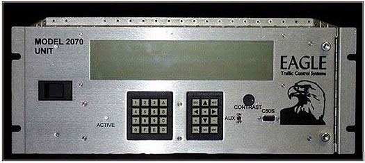
Source: FHWA.
As the upgrade to the 170, the 2070 provides additional and higher-speed communication ports with industry-standard connector types (Serial DB9 and Ethernet RJ45), a higher-speed processor that runs a real-time operating system (OS-9), additional memory, and a back-lit liquid-crystal display (LCD) display. A variety of optional components are available, including a module that allows a 2070 controller to be installed in a NEMA cabinet.
The 2070 controller platform provides serial and Ethernet interfaces with native protocol support. (Assuming software that is capable of supporting Ethernet, there is no need for serial-to-Ethernet encapsulation on a 2070, unlike the 170.) RJ45 Ethernet and direct fiber-optic Ethernet modules are available.
The 2070 is a popular and successful controller platform for a variety of agencies. Due to the number of currently installed 2070s, equipment and spare parts will likely be available for purchase for many years to come. The back-lit LCD display is a significant improvement over the 170's LED display, but can be difficult to view in direct sunlight conditions. A wider variety of firmware options are available for the 2070 than for the 170, including options from developers that are completely independent from hardware manufacturers and vendors.
NEMA
The National Electrical Manufacturers Association (NEMA) standard and its versions (TS1, TS2 Type 1, TS2 Type 2) have been in existence for more than 30 years. The standard covers the controller-cabinet interface through three connectors (A, B, and C) and standardizes some nomenclature and controller terminology, although not covering all features and functions of a controller. NEMA controllers are procured as a package of controller firmware and hardware. NEMA controllers support both serial and Ethernet/IP communications, with newer versions supporting both natively.
ATC
The Advanced Transportation Controller (ATC) standard began in 2005 as the successor to the 2070 standard. Version 5.2b is currently approved as a joint standard of American Association of State Highway and Transportation Officials (AASHTO), Institute of Transportation Engineers (ITE), and NEMA. Departing from the 170 and 2070 standards, the ATC focuses on the functionality and Application Programming Interface (API), or the hardware-level interfaces for communications to peripheral devices, such as serial ports, Ethernet ports, USB drives and flash memory arrays, and displays. The functionality of the traffic controller is thus encapsulated in an engine board that runs the Linux operating system. The ATC standard clearly defines the physical and functional requirements of the engine board. The ATC standard also defines the general requirements for a host module mated to the engine board. The host module can be packaged by a vendor to meet the requirements of a specific application (e.g., a NEMA shelf-mount controller or a module to plug into a 2070 controller).
The ATC controller standards require that the controller enclosure support a minimum of one communication module slot that has a form factor that conforms to the requirements of the 2070. This means that the ATC controller can support many different communications modules including serial, fiber optic, wireless, etc.
The most common ATC firmware application is a traffic controller. The real-time operating system environment is also well suited for many ITS applications. Algorithms can be stored and run locally in a continuous fashion, enabling such applications as queue-end warning systems, border wait time measurement systems, or traffic incident detection algorithms.
Return to top ↑
Dynamic Message Signs
Dynamic message signs (DMSs) are used to disseminate relevant information to motorists along the roadway. DMS is the preferred term according to the National ITS Architecture, although some jurisdictions still use other terms interchangeably, such as variable message signs (VMSs) or changeable message signs (CMSs). DMS are large, electronic signs that overhang or appear along major highways and are typically used to display information about traffic conditions, travel times, construction, and roadway incidents.
The largest of these signs are mounted overhead on a gantry. Overhead signs can be made to provide maintenance access from the front, from the rear, or from the side using a walk-in configuration. Figure 19 shows an overhead DMS currently installed along a highway in Ohio.
Figure 19. Overhead DMS
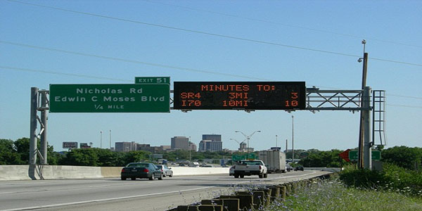
Source: Ohio DOT.
Traditional DMSs are monochrome and are limited to three lines of only text (a practical limitation as DMS standards do not preclude using more than three lines). Multiple, three line messages can be cycled to increase the amount of information a sign can provide. Due to the time it takes a motorist to read and process this information, no more than two cycles (or two phases) are usually presented at any given time.
DMS operation is governed by the sign controller. Messages can be updated automatically to the sign controller by the central system in response to current traffic conditions, or remotely updated to the sign controller in special circumstances, such as a lane closure. Messages can be stored on a central server, created on-demand by the central server (or operator) based on a template, or contained in the sign's internal message library. Most fixed DMSs (i.e., nonportable) use a wired communication format (e.g., Ethernet).
In most DMS applications, information on the sign is presented and seen by motorists via the illumination of LEDs. Typically, LEDs are positioned in an array where each array illuminates analogous to a pixel on a computer monitor. Internal hardware and software drivers are used to illuminate each individual LED (or pixel). Text and messages are formed by illuminating LEDs in a specific configuration. Most DMSs allow for operators to adjust the size and spacing of message fonts depending on the size of the sign and its application. Agencies should select a sign that is the appropriate size to display the types of desired messages.
Newer DMSs offer a display known as full matrix. This type of display allows for the incorporation of images or pictograms. Figure 20 shows an example of a roadside-mounted DMS with a full matrix monochrome display.
Figure 20. Full Matrix Monochrome DMS
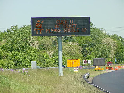
Source: Ohio DOT.
Full color, full matrix DMSs are also available and provide a robust display format on which to provide traveler information. They provide the ability to more closely emulate road shields and other Manual on Uniform Traffic Control Devices (MUTCD)-compliant graphical elements. Reproducing graphical elements that drivers are accustomed to seeing may help mitigate the issue of driver distraction by reducing the amount of time a driver needs to read and process the information contained on the DMS. Figure 21 shows a full color, full matrix DMS with walk-in maintenance access.
Figure 21. Full Matrix Color DMS
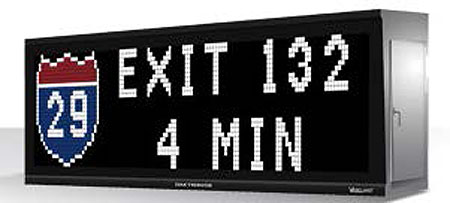
Source: Daktronics, Inc.
Portable DMSs differ from fixed DMSs in several ways. The first and most obvious difference is that these signs are designed to be transportable, making them ideal for temporary applications, such as work zones. These signs are much smaller than most fixed DMSs and are mounted on a portable trailer that can be towed behind vehicles with a standard trailer hitch. Figure 22 shows a portable DMS deployed in a work zone.
Figure 22. Portable DMS
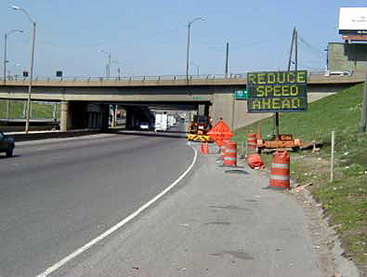
Source: FHWA.
Power and communications are also different for portable DMSs, as there is usually no permanent source nearby for either of these necessities. On-board batteries power the sign and communications equipment. Solar panels, which charge the batteries and therefore prolong the deployment period, are mounted to the top of the sign. The size of the batteries and solar panels are usually calculated based on the geographic area in which the sign will be deployed, due to varying solar conditions.
Cellular data communications are used to communicate with the portable DMS via an on-board cellular modem. This enables the sign operator to change the displayed message and monitor the equipment status. GPS units are also installed in the units to assist operators with locating the signs.
Figure 23. Standard Enclosure
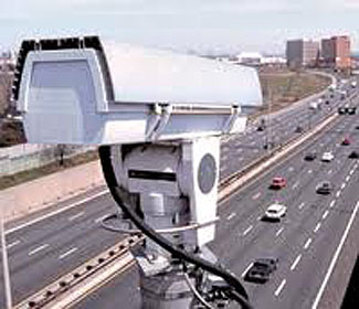
Source: FHWA.
Return to top ↑
Video Cameras
Video cameras are used in a variety of transportation applications. A camera system comprises the camera, housing, monitor/recorder, central control system, and supporting infrastructure, such as the pole on which the camera unit is mounted, power, and communications equipment. Cameras are typically mounted at a height of 35 feet by 50 feet (extending as high as 100 feet) and provide the ability for operators, watching on the monitoring screen, to pan, tilt, and zoom the camera. Pan and tilt capabilities are a function of the camera's housing or the unit to which the housing is mounted. Traffic management applications generally require a zoom capability of between 18x to 22x with typical cameras offering upwards of 35x.
Traffic cameras are typically housed in two types of enclosures: standard and dome.15 The type of enclosure used will have some impact on the capabilities of the camera and the required maintenance. The function of the enclosure is to protect the camera equipment from both the environment and vandalism.
Standard enclosures are typically mounted on a pan/tilt unit to provide the ability to move the camera both horizontally and vertically. This ability allows the operator to precisely position the camera to view all areas surrounding the camera. The interface to the camera typically provides the option to designate predetermined positions, or presets, of the camera to enable quickly returning to areas of interest. The cameras can also be configured to cycle through multiple presets or continually pan/tilt, although this function isn't commonly used in traffic monitoring applications.
Figure 24. Dome Enclosure
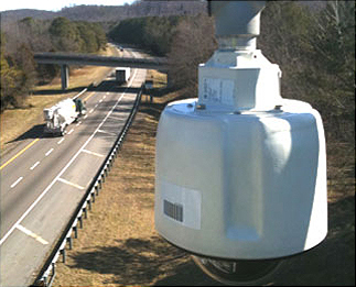
Source: FHWA.
Dome enclosures are slightly more robust than standard enclosures. The pan/tilt capabilities are better than most standard enclosures, providing a 360-degree view of the surrounding area. These enclosures are highly compatible with lowering devices, which makes them easier to maintain. The moving parts are protected behind the dome enclosure, and they provide better aesthetics than standard enclosures. Newer standard-style enclosures can provide 360-degree pan/rotation and 90- to 360-degree tilt, making them comparable to dome enclosures.
Video image quality is a product of resolution, frame rate, and compression type. Standard definition video cameras provide a resolution (pixels/inch) and frame rate (frames/s) of 720x486 and 29.97 (National Television System Committee) with an aspect ratio of 4:3. High definition video cameras provide a resolution of either 1280x720 (720p) or 1920x1080 (1080i/p) and frame rates ranging from 23.98 to 60 with an aspect ratio of 16:9. The video is compressed prior to transmitting back to the central control system to reduce the amount of bandwidth required for each camera (e.g., MPEG-4). This is accomplished via a combination of spatial image compression and temporal motion compression. Compression offers a tradeoff between video quality and required data rates. More compression results in decreased video quality but lower required bandwidth; and less compression results in better video quality but higher required bandwidth.
Environmental Conditions
Environmental conditions remain one of the biggest challenges associated with traffic camera operation, but technological advancements in camera systems continue to provide improved mitigation. Wipers (standard enclosures), demisters, and special lens coatings can help reduce the effects of rain and fog by clearing the enclosure's viewing window. Built-in heaters can help preserve equipment and reduce the effects of low temperatures in cold climates. Lightning strikes can be mitigated through proper installation of surge protection devices and proper grounding of all equipment associated with the camera. In extreme cases, lighting rods may need to be installed near the cameras.
Cameras can operate at night and in low-light conditions but with some limitations. Most new cameras are typically equipped with auto iris functions that automatically adjust to changing light conditions. Despite this, glare from vehicle headlights can make it difficult to provide an effective low-light image. Monochrome cameras typically perform better in low-light conditions than color cameras. Some cameras can automatically switch from color to monochrome in low-light conditions.
IP Cameras
Traditionally, cameras deployed for ITS applications provided analog signals. In order to transport the video images, the analog signals were converted to digital signals using video encoders (or codecs). These video encoders would also provide video compression, to minimize bandwidth utilization, and Ethernet communication capability. The features of analog-to-digital video conversion, video compression, and Ethernet communication capability used to exist in a separate unit outside of the video cameras. These features have since been integrated into the camera itself. A camera with these integrated features is referred to as an IP camera.
This type of camera is popular in traffic-monitoring applications because it reduces the amount of equipment and connections required to implement a camera and view the live feed. The digital output from the camera can be easily transmitted via the Internet or private communications network back to a central monitoring location (e.g., the TMC). The digital stream can then be viewed on multiple monitoring screens and easily shared with media agencies or the public. IP cameras with built-in cellular wireless communications can even allow for portable camera deployment. The Web-based nature of IP cameras makes for a very versatile video platform for ITS applications as the cameras can connect to a network very easily. One of the drawbacks of using IP cameras is the control latency. Low-latency serial connections typically offer superior performance for operator initiated pan-tilt-zoom functions over their IP counterparts. The result is a delay between the time an operator initiates the control activity and when the repositioned image is displayed, which can make manually positioning the camera difficult.
On-Vehicle Cameras
Advancements such as IP camera capabilities can be combined with advancements in physical components to solve specific applications. One such application is on-vehicle cameras. In public transit, there is a need to monitor on-board activities for a variety of reasons, safety in particular. On-vehicle cameras use compact, rugged enclosures that typically contain some kind of vibration damping technology to mitigate the effects of bumps in the road and vehicle movements. PoE is another innovation that supports this kind of deployment, allowing the camera unit to be powered through the same cable it uses to communicate the video feed. Video is stored on a recorder unit located within the vehicle.
Return to top ↑
Road Weather Information Systems
The key supporting technology behind RWIS is the environmental sensor stations (ESS). An ESS is used on a fixed roadway location with one or more sensors measuring atmospheric, surface (i.e., pavement and soil), and/or hydrologic (i.e., water level) conditions. The stations are typically deployed as field components of a RWIS. Data collected from environmental sensors in the field is stored onsite in a remote processing unit (RPU) located in a cabinet. In addition to the RPU, cabinets typically house power supply, battery back-up devices, and other supporting infrastructure, such as communications equipment. In addition to the communications options outlined in the communications section of this module, satellite communications can be used to connect the ESS to the central system. Typically, ESSs are connected to the central system through one of the communications options listed in the communications section of this module. The remote location of some ESS may preclude the use of traditional communications options, such as cellular data, since coverage may not be available. In these cases, satellite communication links have been established to connect the stations back to the central system. This section examines the technical components of an ESS (a typical configuration is shown in Figure 25) as implemented in the FHWA's Road Weather Management Program.16
Figure 25. ESS
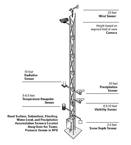
(Extended Text Description: This is an illustrated diagram of a Road Weather Information System (RWIS). The RWIS is a metal tower that has many different sensors mounted onto its sides. From bottom to top, sensors mounted onto the system include a snow depth sensor (3.5 feet), a Temperature Dewpoint Sensor (5-6.5 feet), a Visibility Sensor (6.5-10 feet), a Precipitation Sensor (10 feet), a Radiation Sensor (10 feet), and at the top, a camera, and a wind sensor (33 feet). The height of the camera is based on the required field of view. Road Surface, Subsurface, Flooding, Water Level, and Precipitation Accumulation sensor are located away from the tower, Pressure Sensor in the RPU.)
Figure 26. Wind Vane
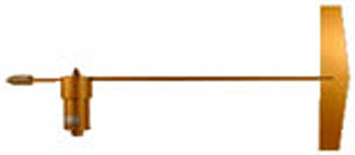
Source: FHWA.
Figure 27. Propeller Wind Vane
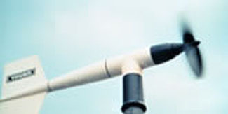
Source: FHWA.
Air Sensors
Wind
Wind vanes are employed to determine the direction from which wind is blowing. A conventional wind vane indicates wind direction with a tail fin mounted on a horizontal shaft that is attached to a vertical axis. The tail causes the wind vane to rotate in the horizontal plane. Wind speed is typically measured by anemometers with propellers or cups. A vane-oriented propeller anemometer uses two to four blades, which rotate about a horizontal shaft, and a vane attached to the shaft to indicate direction.
Rotating cup anemometers have three to six hemispherical cups that revolve around a vertical axis. Speed is calculated based upon the rotation rate of propeller blades or cups. Wind speed can also be determined with nonmechanical sensors, such as hot wire and sonic anemometers. Hot wire anemometers ascertain the degree of cooling of a heated metal wire, which is a function of air speed. A sonic anemometer gauges wind speeds based upon properties of wind-borne sound waves. A wind speed and direction sensor, or anemometer, should be positioned 33 feet above ground level. The wind direction sensor should be set on true north, rather than magnetic north.
Pressure
Mercury and aneroid barometers are employed to detect atmospheric pressure or the pressure due to the force of gravity on air molecules in a column of air. Because they are more accurate than mercury barometers, aneroid barometers are typically used in meteorological applications. An aneroid barometer contains an aneroid cell—a sealed, flexible metal box or a pair of thin circular disks—that expands or contracts as atmospheric pressure changes.
Temperature/Dew Point Sensor
Air temperature can be measured with liquid, gas, or electrical thermometers. Electrical thermometers, which are normally used in automated sensor stations, contain metal wires that exhibit increased resistance to electrical current as the temperature rises. Platinum and copper are commonly utilized due to a nearly linear relationship between resistance of these materials and temperature. Electrical thermometers, also known as resistance thermometers, and thermoelectric thermometers provide accurate readings over a wide range of temperatures.
Relative humidity, a measure of air's water vapor content, can be measured by three types of hygrometers. Dew point, capacitor, and electrical hygrometers detect humidity by sensing changes in a substance caused by moisture. An air temperature/dew point sensor should be housed in a radiation shield and mounted 5 to 6.5 feet above the ground. The sensor should be on a boom extended at least 3 feet from the tower in the predominant wind direction.
Precipitation Sensors
Figure 28. Tipping Bucket Rain Gauge
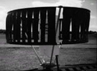
Source: FHWA.
Precipitation Sensor/Precipitation Accumulation Sensor
Precipitation measurements are made with rain gauges that sense precipitation type, measure the amount and rate of rainfall (or the liquid equivalent of snow or sleet), as well as determine the start and end times of a precipitation event. Tipping-bucket rain gauges and weighing rain gauges are commonly used in ESS. In tipping-bucket gauges, a cylinder collects and funnels rainfall into a small bucket that holds 0.01 inches of water. In climates with frequent snowfall, the bucket is heated and equipped with a wind shield. When it is full, the bucket tips and empties the water while another bucket is lifted into position under the funnel. Every time a bucket tips an electrical contact is closed sending a signal to a recorder. Weighing rain gauges are capable of measuring all types of precipitation without heaters. Precipitation is funneled into a bucket that is weighted to assess amounts. These gauges require more maintenance than tipping-bucket gauges. Float-type rain gauges use a float on the water surface to measure the amount of liquid precipitation. Rain-intensity gauges or rate-of-rainfall gauges measure the instantaneous rate at which rain falls onto a surface. A hotplate snow gauge consists of two heated plates that are used to estimate snowfall mass by measuring the power to melt and evaporate snow on the upward-facing plate. The gauge compensates for wind effects by subtracting the power on the downward-facing plate. The hotplate snow gauge measures the liquid equivalent snowfall rate from 0.01 to 1.00 inch/hour.
Snow Depth Sensor
A snow depth sensor emits an ultrasonic or infrared pulse and measures the time it takes to travel to the snow surface and return to the sensor. An internal algorithm adjusts the time, based on the air temperature, and converts it into a distance. A study by the National Weather Service found that this technology shows promise as an objective tool for measuring snow accumulation where human observations are not possible. A snow depth sensor should be installed perpendicular to the surface at a height of approximately 3.5 feet. The sensor should have an unobstructed view of the target and should be mounted to avoid vibrations.
Figure 29. Road Surface Sensor
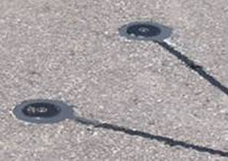
Source: FHWA.
Road Surface Sensor
Surface sensors measure pavement conditions (e.g., temperature, dry, wet, ice, freeze point, and chemical concentration). There are two basic types of surface sensors: active and passive. Active sensors generate and emit a signal, and measure the radiation reflected by a targeted surface. Passive sensors detect energy radiating from an external source. Passive pavement temperature sensors are normally buried in the road surface. These sensors are designed with thermal properties similar to pavement so that they are heated and cooled at the same rate.
Pavement condition can be monitored with sensors embedded in road surfaces, friction-measuring devices, cameras, and microphones. As shown in Figure 29, embedded sensors typically distinguish between two or three pavement states (e.g., dry or wet). The surface of an active pavement condition sensor is cooled below ambient air temperature. If pavement moisture is present, dew or frost will form on the cooled surface. This type of sensor can also be used to assess the effectiveness of road treatment chemicals and determine the temperature at which pavement moisture will freeze.
Nonintrusive pavement condition sensors are available. These sensors are installed on a tower above ground and emit microwaves or infrared beams from an overhead transmitter. Microwaves reflect off of the water surface and the road surface if moisture is present on the pavement. A receiver detects the pattern created by the reflections to compute the thickness and salinity of a film of water. The infrared sensor provides road surface conditions as well as the friction level of road surface, using a specific friction algorithm.
Figure 30. Stilling Well
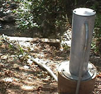
Source: FHWA.
Subsurface Sensor
Subsurface conditions (e.g., soil temperature, soil moisture, and freeze/thaw cycles) may be detected with a soil thermometer or geothermometer, which measures values at various depths. These conditions characterize the transfer of heat between the soil and the pavement. Subsurface temperature and moisture sensors should be installed at a depth of 12 or 18 inches. The installation location should be representative of subgrades in the area to include the presence or absence of water, similar soil types, and pockets of foreign materials.
Water-Level Sensor
Various hydrologic sensors detect water levels in streams and rivers, and tide levels to assess flood and storm surge hazards. Ultrasonic water-level sensors make use of acoustics or sound waves to measure the distance from a transducer to the water surface. Stilling wells contain float sensors to measure water levels. The float is typically enclosed in a pipe or cylinder, which protects the sensor and allows the free movement of water. Tide gauges may be used to measure storm surge caused by a tropical storm. These gauges operate in a manner similar to stilling wells to measure the height of tide. Standpipe masts are vertical pipes ranging from 3 to 12 inches in diameter and up to 10 feet tall.
Visibility and Radiation Sensors
Figure 31. Visibility Sensor
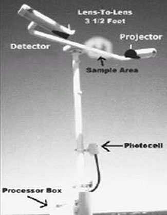
(Extended Text Description: This is an example of a Visibility and Radiation Sensor. This sensor is made up of a long pole with a crossbar mounted at the top. There are multiple devices installed onto this frame. Starting at the base, there is a Processor Box. On the lower half of the post is the photocell. Mounted on the end of the crossbar is a projector and detector on the other end. The air sample area is located in between the projector and the detector. The distance between the two lenses is 3 ½ feet.)
Source: FHWA.
Visibility Sensor
Visibility can be reduced by various weather phenomena including fog, heavy precipitation, drifting snow, and wind-blown dust. Visibility distance can be measured directly with sensors or remotely via video cameras. Objects suspended in the air—such as minute water droplets forming fog—scatter energy. Visibility sensors detect the amount of scattered light to compute visibility distances. A forward-scatter visibility sensor has a projector that emits a pulsed flash of light in a cone-shaped beam. A detector is positioned 33 to 70 degrees from the projector axis, such that the beam does not fall directly on the detector lens. Thus, the detector senses only the light scattered by fog or dust. Backward-scatter visibility sensors have aligned projectors and detectors, and operate in a manner similar to forward-scatter sensors. Visibility sensors should be installed at a height of 6.5 to 10 feet to represent driver-level conditions. Optical sensors should be installed to prevent the sun and stray light sources from entering the receiver element.
Camera
Visibility distance can be discerned by aiming a video camera at objects at known distances, such as roadside signs with flashing beacons. When cameras are used for visibility measurements, the camera should be installed as close as possible to the driver's level of view.
Radiation Sensor
Solar radiation sensors should be installed at least 10 feet from the surface to avoid radiation from reflective surfaces, debris contamination, and shading from obstructions. Both visible and infrared cameras should be installed where they are able to obtain a clear line-of-sight without interfering with the operation of other sensors.
Return to top ↑
Connected Vehicle Technologies
Connected vehicle technology refers to the technology that enables connected vehicle applications. Module 13 of this ePrimer discusses connected vehicles and connected vehicle applications in detail. This section focuses on some of the specific technologies that enable these connected vehicle applications. These technologies leverage the potentially transformative capabilities of wireless communication to make surface transportation safer, smarter, and greener. The trend is inevitable; connected vehicles are the new wave of intelligent transportation technology with the potential to address up to 80 percent of unimpaired driver crashes while potentially reducing the estimated 4.8 billion hours Americans spend in traffic each year.17
This video link provides an overview of the connected vehicle lifestyle concept.
https://www.youtube.com/watch?v=fegzbBhEQjY- content is no longer available.
The USDOT, in cooperation with the automotive industry and other partners, strives toward the goal of enabling networked, wireless communications among all vehicles types and is promoting development and deployment by the private and public sectors.
RSE and OBE
Roadside equipment (RSE) represents the static infrastructure component of the connected vehicle. On-board equipment (OBE) represents the in-vehicle component of the connected vehicle. RSE collects vehicle data through communication with the vehicle's complementary OBE. There is still no standard specification for connected vehicle RSE or OBE, although there have been several implementations and test beds demonstrating the various capabilities of a connected vehicle.
The following video introduces the concept of using connected vehicle technology at intersections.
www.its.dot.gov/communications/media/3ica_dsrc.htm
Sensors mounted on the vehicle can detect the presence and movements of other nearby vehicles. On-board processors can merge the driver vehicle's information, such as speed, with the speeds, locations, and trajectories of nearby vehicles to identify and warn of unsafe conditions. The following video elaborates on this concept.
www.its.dot.gov/communications/media/2ivhw.htm
This next video provides several examples of actual connected vehicle demonstrations.
https://www.youtube.com/watch?v=FLjyW_IqszY
The concept can even be extended to pedestrians. Arizona implemented a test project that connected users' smartphones with intersection infrastructure so that the crosswalk crossing status could be dynamically displayed on the users' phones (along with audible alerts). Pedestrians could use this interface to request an extension to the crossing time.18
5.9GHz Dedicated Short-Range Communications
DSRC technologies were developed specifically for vehicular communications and have been closely associated with connected vehicle (and its predecessor) initiatives. In the United States, DSRC is used generically to refer to communications on a dedicated 5.9GHz frequency band using the wireless access in vehicular environments (WAVE) protocols defined in the IEEE 1609 standard and its subsidiary parts. These protocols build on the established IEEE 802.11 standards for Wi-Fi wireless networking. Standard messages for DSRC are described in the Society of Automotive Engineers (SAE) J2735 standard. These standards continue to evolve, but have provided the basis for most connected vehicle DSRC demonstrations.19
DSRC is uniquely suited to mobile vehicular applications needing high bandwidth and low latency in short-range communications on the order of a few hundred meters. Security is managed through a certificate management scheme that issues new certificates to each radio at regular intervals. Radios are deployed in vehicles and in roadside equipment to provide vehicle-to-vehicle and vehicle-to-infrastructure (or infrastructure-to-vehicle) communications. DSRC is still relatively early in its development and application life cycle. Although there are currently no operational deployments, several small networks have been established to support development and test in Florida, New York, California, and Michigan. Similar test beds are being installed in Edmonton and Vancouver, Canada. The most comprehensive, in terms of scale and objectives, is the USDOT Safety Pilot in Ann Arbor, MI.
The following video presents an overview of how DSRC could be used to monitor traffic conditions using the connected vehicle technology. Click the link to watch the video. www.its.dot.gov/communications/media/1probe.htm
Return to top ↑
Summary
The intention of this ePrimer module is to promote an understanding of the various technologies used in ITS applications. The sections are organized to encapsulate and group the various physical components of ITS so that the different types of technologies can be compared and understood. By combining an understanding of the role of a specific ITS component with knowledge of the strengths and weaknesses of comparable technologies that can fill that role, agencies can be empowered to make informed decisions in their future ITS deployments.
It is also important to note that effective ITS applications are those that begin with clearly defined goals and requirements. What can often occur in high technology environments, such as the ITS domain, is a tendency to let the technology be the driver of the application. That is, agencies may focus too much on matching the capabilities of the technology to the transportation problem, rather than starting with the transportation problem and letting those requirements drive the application of technology.
Future Considerations
The ITS industry is ever evolving. This section examines a few of the issues and trends that could shape the future of supporting ITS technologies.
Technology Trickle-Down Effect
Although many ITS applications involve the development of proprietary systems to solve specific problems, tremendous opportunities have been realized through the proliferation of technological advancements in other sectors. Communications is a great example of an area benefitting from this technology trickle-down effect. Cellular service providers have continued to increase network coverage, bandwidth, and download speeds. This increased coverage and throughput has had a great enabling effect on ITS applications by providing an unprecedented level of connection between the TMC and field devices. Traffic controllers at remote intersections can now be connected centrally at a low cost. Bandwidth is sufficient for the implementation of portable video cameras used in work zones.
The security and surveillance industry provides another area where developments could be ported to ITS applications. A panamorph lens, which can be attached to any video camera, provides a distorted image that captures a 360-degree view of an area simultaneously. Software, which can take the distorted image and flatten it to provide simultaneous views of all sides of the camera, is available. The following example explains the benefits of this type of camera.
Figure 32. Panamorph Lens Image Flattening
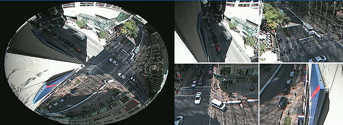
(Extended Text Description: This is a collection of images demonstrating the panamorph lens image flattening. The large image on the left is in a rounded oval, showing the curved image of an urban setting. The right side is split into four quadrants with one image in each. Each image shows an urban street scene with traffic on roadways, and sidewalks, surrounded by buildings.)
Source: ImmerVision.
An installation of a camera with this type of lens at an intersection could provide the ability to monitor all approaches at once. Combine this with existing traffic video imaging processing algorithms and the potential exists to fully monitor an intersection with one camera. ITS will continue to benefit from technology developments in other industries.
New Data Sources
Another emerging trend is the availability of data from nontraditional sources. Cell phones and smartphones, for example, provide a vast amount of data that was not previously available. As discussed in a previous section, traffic information can be derived from motorists using their cell phone in their vehicle. The evolution of this technology could lead to the motorist simply needing to have their cell phone with them (rather than actively using it) in order to obtain traffic data.
Smartphones provide a unique opportunity that is only starting to become realized. In-device smartphone mechanisms, such as gyroscopes and accelerometers, could provide information on road surface conditions. These are the same devices used by agencies applying the International Roughness Index (IRI) in their road asset management programs. Research has only just begun investigating whether these smartphones could effectively replace existing, costly, data-collection equipment.20
Social media provide a wealth of real-time traveler information that is predominantly untapped. Monitoring and interpreting social media have become a huge business in the private retail sector. It is likely these same tools and concepts could be implemented in the transportation sector. Crowdsourcing information through the variety of social media streams available may provide the opportunity to enhance, or even replace, costly existing systems.
Standards
Standards in ITS are extremely important. ITS applications require a high level of integration among components. Standards reduce the need for reliance on specific equipment vendors and customized one-of-a-kind software by providing standardized interfaces that enable the integration of multiple components from multiple manufacturers.
The National Transportation Communications for ITS Protocol (NTCIP) is one such ITS-enabling standard. The NTCIP is a family of standards that provides both the rules for communicating (called protocols) and the vocabulary (called objects) necessary to allow electronic traffic control equipment from different manufacturers to operate with each other as a system. The NTCIP is the first set of standards for the transportation industry that allows traffic control systems to be built using a mix-and-match approach with equipment from different manufacturers. To assure both manufacturer and user community support, NTCIP is a joint product of the National Electronics Manufacturers Association, the American Association of State Highway and Transportation Officials, and the Institute of Transportation Engineers.21
One of the difficulties is that these standards need to continue to evolve as technology evolves. The speed of hardware processors and communications continue to increase, meaning both the hardware manufacturers and the standards setters must constantly adapt to help ensure capitalization of advancements in combination with integration.
Another issue that needs to be monitored is the proper adherence to standards. Often, devices manufactured to a specific standard have difficultly integrating with other devices of the same standard. It needs to be understood that standards are not necessarily perfect or all encompassing. The implication of this is an increased level of integration testing required. Although the intent is for standards to consistently improve, agencies are wise to consider this issue in future implementations.
Return to top ↑
References
Return to top ↑